
Measuring Predictive Accuracy
Raw data (only for illustration)
| X | Y | Forecast Value |
|---|---|---|
| 1 | 0.3324 | 1 |
| 2 | 2.9232 | 2 |
| 3 | 1.4348 | 3 |
| 4 | 4.0073 | 4 |
| 5 | 3.7612 | 5 |
| 6 | 5.1456 | 6 |
| 7 | 8.1008 | 7 |
| 8 | 8.3195 | 8 |
| 9 | 8.4495 | 9 |
| 10 | 10.9755 | 10 |
| 11 | 12.1784 | 11 |
| 12 | 13.6671 | 12 |
| 13 | 14.6767 | 13 |
| 14 | 17.7715 | 14 |
| 15 | 17.1683 | 15 |
| 16 | 17.0177 | 16 |
| 17 | 19.6758 | 17 |
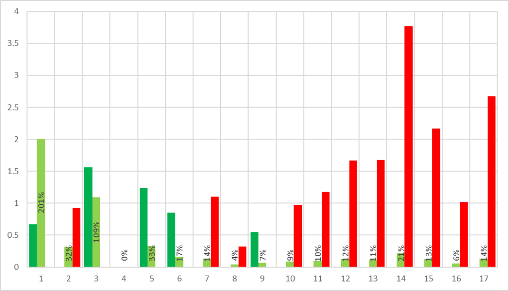
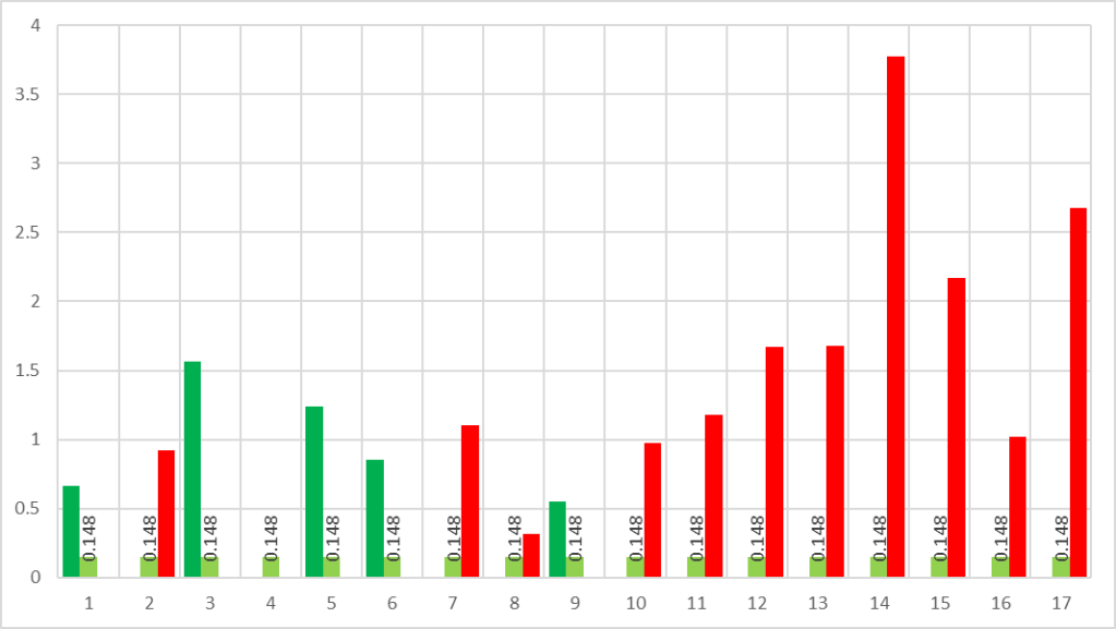
Black Square = Forecast Value
Yellow Circle = Actual Value
Green Box = Forecast value above Actual Value
Red Box = Forecast value below Actual Value

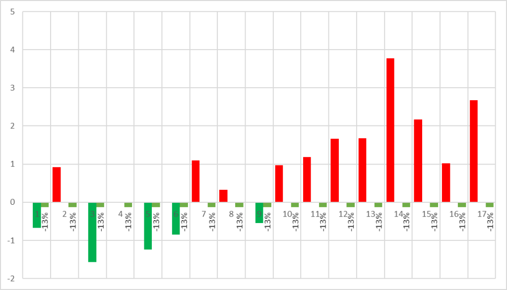
Average/Mean Error (ME/AE)
ps. Value different between data point; affect by positive/negative cancel each other.
SUM( Actual Value - Forecast Value ) / number of data pointStep 1. Identify the delta between Actual Value and Forecast Value


Step 2. Sum all delta
Step 3. Divide the delta with number of data point

Can be use to identify
- AE < 0, forecast line above actual line; over-predict
- AE > 0, forecast line under actual line; under-predict
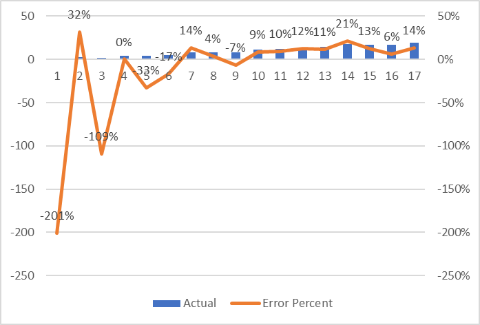
Mean Percentage Error (MPE)
ps. Value percentage different between data point; affect by positive/negative cancel each other.
SUM (
     ( Actual value - Forecast Value ) / Actual Value
    ) / Number of data pint
Step 1. Use the delta from above and divide by actual value to obtain “Error Percentage”

Step 2. Sum all percent
Step 3. Divide the percent with number of data point
Can be use to identify
- MPE < 0, forecast line above actual line; bias high
- MPE > 0, forecast line under actual line; bias low
Mean Absolute Error (MAE)
ps. Distance between data point.
SUM(
     ABS ( Actual Value - Forecast Value )
   ) / number of data point
Step 1. Identify the actual delta/distance between Actual Value and Forecast Value
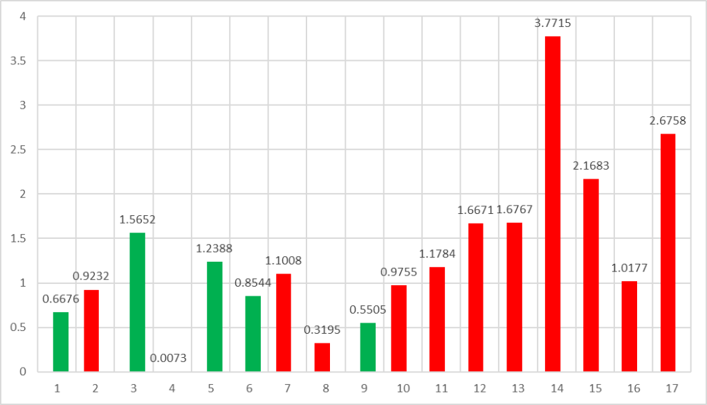
Step 2. Sum all distance
Step 3. Divide the percent with number of data point

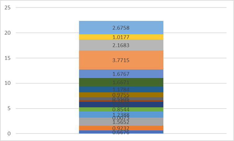
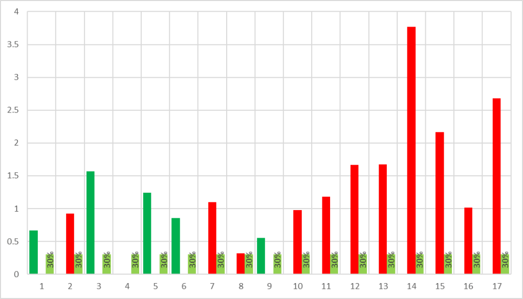
Mean Absolute Percentage Error (MAPE)
ps. Distance percentage between data point; benefit is to compare with data having different scale.
SUM(
     ABS ( Actual Value - Forecast Value ) / Actual Value
   ) / number of data point
Step 1. Use the delta from above and divide by actual value to obtain “Error Percentage”
Step 2. Sum all percent
Step 3. Divide the percent with number of data point
Root Mean Square Error (RMSE)
ps.
SQRT(
     SUM(
         ( Actual Value - Forecast Value ) ^ 2
        )
    ) / number of data point
Step 1. Use the delta from above and power 2 to obtain “Error Squared”

Step 2. Sum all squared delta
Step 3. Divide the squared delta with number of data point, square root it again
Mean Absolute Scaled Error (MASE)
ps. A metric to tell a model is performing better than flipping coin.
MAE / MAE of (eg. k-step ahead naive forecast)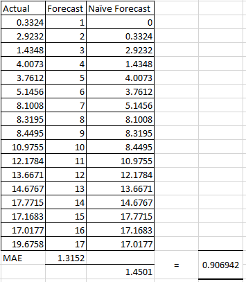
Can be use to identify
- MASE < 1, better than naive forecast
- MASE > 1, worst than naive forecast
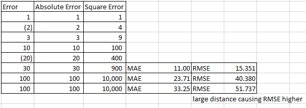
MAE VS RMSE
| MAE | RMSE |
|---|---|
| measures the average magnitude of the errors in a set of forecasts, without considering their direction | Since the errors are squared before they are averaged, the RMSE gives a relatively high weight to large errors. This means the RMSE is most useful when large errors are particularly undesirable. |
Data Partition
How to tell a model accuracy? Say after trained a model, performed above measurement and got RMSE value, how to tell is the model performing good? or bad? or overfitting? A comparison is needed and that introduced data partition. Portion of data is reserve to validate a model metric.
ps. One point to think off, classification/regression can split data randomly for train/test but time series forecasting only can split by sequence.
After the validation, data split-ed must be recombine back as one. The new model must be trained with past and latest data, to cover everything.
R
library(forecast)

quakes <- ts(data=Earthquakes$earthquakes)

plot(quakes)

train_quakes <- quakes[ 1 : ( 0.8 * length( quakes ) ) ]
test_quakes <- quakes[ -c( 1 : ( 0.8 * length( quakes ) ) ) ]

ses_quakes <- ses(train_quakes,
                  initial="simple",
                  h=length(test_quakes))

holt_quakes <- holt(train_quakes,
                    initial="simple",
                    h=length(test_quakes))

accuracy(ses_quakes,
         test_quakes)

accuracy(holt_quakes,
         test_quakes)
Result:

Cross Validation (Time Series version)

Unlike typical cross validation where “test” is the smallest subset and train will be the remaining set; CV for time series “train” could be the smallest subset. Small portion of data (must according to time sequence) is elected for “train” subset. Models trained and forecasted value will be used in next iteration of model train/selection until all data is fully utilized.
Tutorial 3
Question 1
Crude oil production is defined as the quantities of oil extracted from the ground after the removal of inert matter or impurities. It includes crude oil, natural gas liquids (NGLs) and additives. This indicator is measured in thousand ton of oil equivalent (toe). Crude oil is a mineral oil consisting of a mixture of hydrocarbons of natural origin, yellow to black in color, and of variable density and viscosity. NGLs are the liquid or liquefied hydrocarbons produced in the manufacture, purification and stabilization of natural gas. Additives are non-hydrocarbon substances added to or blended with a product to modify its properties, for example, to improve its combustion characteristics (e.g. MTBE and tetraethyl lead). Refinery production refers to the output of secondary oil products from an oil refinery. Click on the link https://data.oecd.org/energy/crude-oil-production.htm and select TWO countries to analyse the crude oil production (in thousand ton) in the past few years. Split the time series data into training (70%) and testing (30%) data. Use THREE of the following forecasting techniques to perform the forecast:
(a) Moving average or Weighted Moving Average
(b) Modified Moving Average (MMA) or Exponential Moving Average (EMA)
(c) Simple Exponential Smoothing (SES)
(d) Linear, Quadratic or Exponential Trend Model
(e) Holts Method
(f) Holts Winter Method
Evaluate their performances and use the BEST forecasting technique to perform the forecast for the next 5 periods.
Example Answer
Skipped
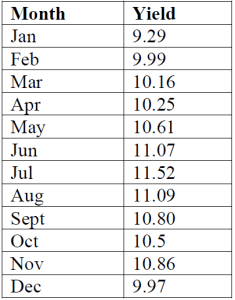
Question 2
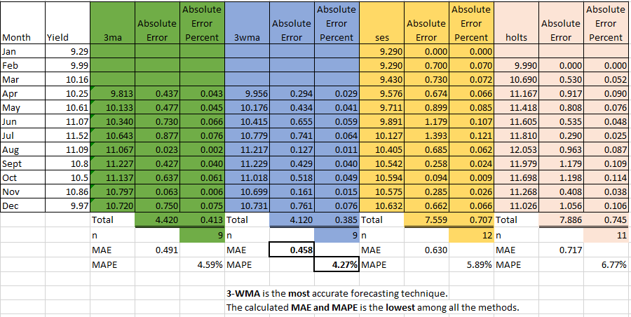
The yield on a general obligation bond for the city of Davenport fluctuates with the market. The monthly quotations for 1999 are as follows:
(a) Find the forecast value of the yield for the obligation bonds for each month using a
(i) three-month moving average.
(ii) weighted moving average (0.50, 0.33, and 0.17 for the most recent, next recent, and most distant data respectively).
(iii) exponential smoothing ( = 0.2).
(iv) exponential smoothing ( = 0.3, β = 0.4).
Example Answer

(b) (i) Evaluate these forecasting methods using MAE/MAD
(ii) Evaluate these forecasting methods using MAPE
Uploaded Answer

Leave a comment