Step 1. Normality of the independent variable distribution test result.

Note that KS test is meant for n > 50 and SW test is meant for n < 50.

Sig value > 0.05 means accept null hypothesis (variable are normally distributed).

Step 2. Collinearity Test.

VIF Value < 10 means there are no multicollinearity.

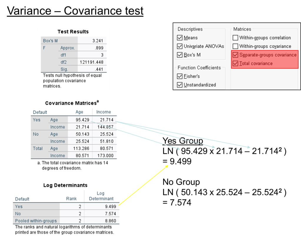
Step 3. Variance covariance test.

Box’s M test (unstable)
H0 : Equal variance-covariance matrix of the independent variable within each group
H1 : There no equal variance-covariance matrix.

Sig Value > 0.05 means there is equal variance-covariance matrix in the independent variable in both categories.

Yes log determinants value is 9, no value is 8; Both are quite close to each other, the variance-covariance matrix is equal.

Step 4. Bring up discriminant analysis dialog box.

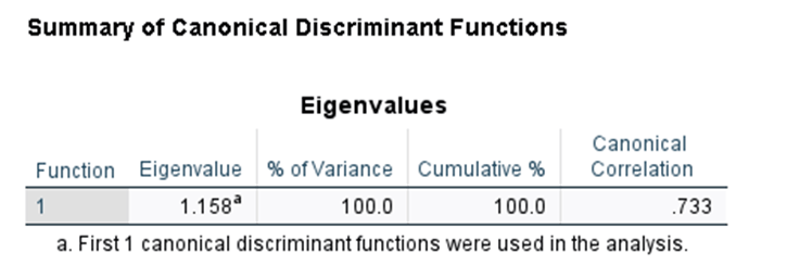
Step 5. Discriminant function explains the variation

Note, only 1 function here as there are only 2 independent variable.

Eigenvalue should be greater than 1.

Canonical Correlation means correlation between independent variable and discriminant function; should be greater than 0.35.

Power(0.733, 2) = 0.537

53.7% variation in dependent variable is explain by the discriminant function.

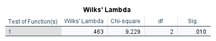
Step 6. Discriminant function significant test.

Sig < 0.05 is significant. Conclusion discriminant function is explains the variance well.

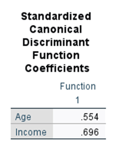
Step 7. Identify most discriminating power.

Income > Age.

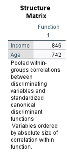
Step 8. Independent variable loading test.

Discriminant loading, should be > +- 0.4

Both age and income has good discrimitary power

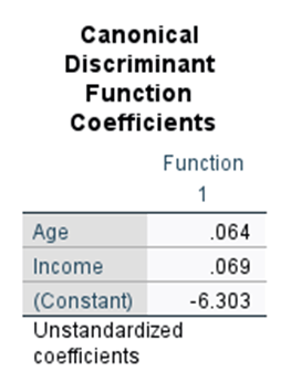
Step 9. Form discrimination function

Z = -6.303 + 0.64(age) + 0.69(income)

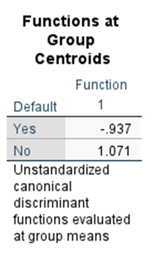
Step 10. Cutting score (Equal prior probabilities)

Zce
= ( Zyes + Zno ) / 2
= (-0.937+1.071)/2
= 0.067

Z < 0.067, classify the individual to Yes

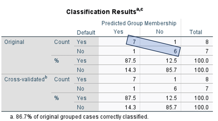
Step 11. Discriminant function accuracy test

Hit Ratio
= (7+6)/15 * 100
= 86.67%

Using equal prior prob, percentage correct classified by chance
= 1 / ( number of group ) x 100
= 1 / 2 x 100
= 50%

Margin up 25%, get 1.25

1.25 * 50
= 62.5%

86.67% > 62.5%, is a good fit model