
Statistical Significance and Power
ps. This is to explain the consequences of making wrong judgement on statistical test.
| H0 is True | H0 is False | |
|---|---|---|
| Accept H0 | Type 2 Error | |
| Reject H0 | Type 1 Error | Power |
Example
Type I error (false positive) involves wrongly diagnosing a healthy person with a medical condition, risking unnecessary surgery.
Type II error (false negative) occurs when a person with the condition is mistakenly deemed healthy, potentially delaying treatment and worsening health outcomes.
Both errors carry serious implications in medical testing, necessitating careful consideration to minimize harm.
Power
We want as large power as possible. But what determine power?

Example, if we were checking on 2 groups of data for single variable, all data point overlap each other (this would mean that there are no relationship to distinguish the data apart, meaning we are accepting null hypothesis of no relation). But how can we tell how many data point is needed to identify accept/reject null hypothesis? by using power.
input power (eg, 0.80) + input alpha (eg, 0.05) + calculate effect size = sample size
Multiple Regression
Statistical technique to analyze relationship between single dependent (criterion) and several independents (predictor).
formula eg.
ŷ = b0 + b1X1 + b2X2 + . . . + bnXn + e
note that b0 meant for setting a baseline value if all of the Xn are zero. Subsequent bn affect how each variable weight in the equation.
Step to form Regression
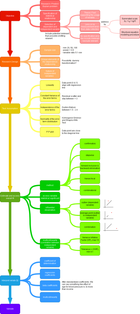
SPSS
Step 1. Import data and configure linearity test setup.


Step 2. Linearity test result.
Income and price are linearly associated.
Step 3. Bring up Regression dialog box.

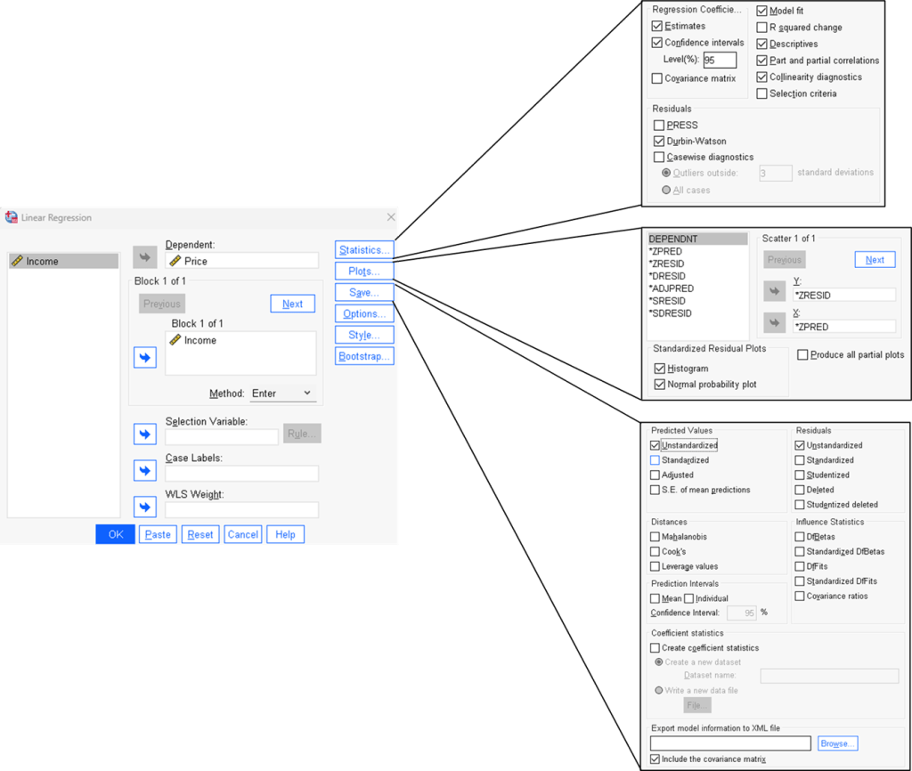
Step 4. Configure all regression setup.
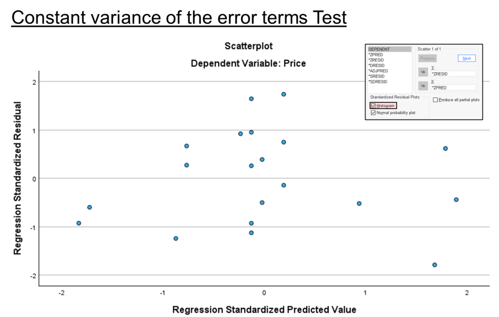
Step 5. Constant variance of the error terms test result.
Predicted residual are randomly distributed, no form of pattern.
Data point fall between value plus minus 3 for both x-axis and y-axis.
Error term has constant variance.
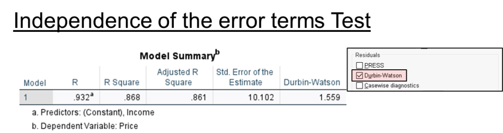
Step 6. Independence of the error terms test result.
DW value between 1.5 ~ 2.4; as the value round become 2.
Independence of the error term is meet.
Step 7. Normality of the error term distribution test result.
P-P Plot shows error term (data point) are close to the diagonal line; normally distributed.
Note that KS test is meant for n > 50 and SW test is meant for n < 50.
Sig value > 0.05 means accept null hypothesis (errors are normally distributed).

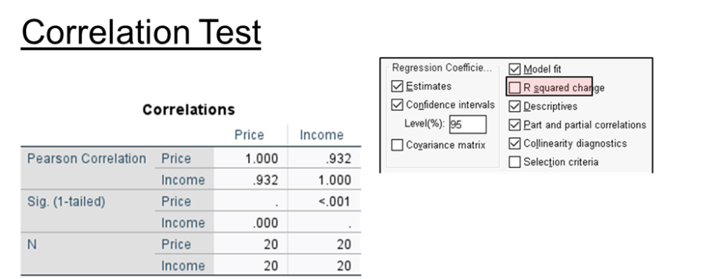
Step 8. Correlation test result.
Relationship between 2 variable. Value can be -1 < r < 1. If value equal to 0 means there is no relation.
Income has strong positive correlation with price, as income increase, price increases.
Sig value < 0.05, correlation is significant and acceptable. Can be use to access the relationship between income and price.
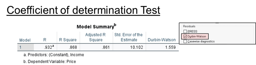
Step 9. Coefficient of determination test result.
R square means coefficient of determination or percentage of variation in the dependent variable that is explained by the independent variable. Value can be 0 < r2 < 1.
86.8% of the variable of price is explained by income.
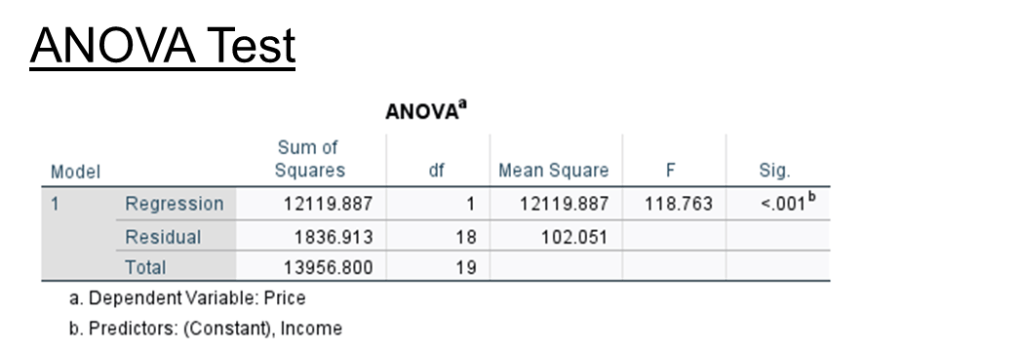
Step 10. ANOVA test result.
The purpose of this test is to tell the model is adequate.
F = mean square of Regression / mean square of Residual.
Sig value < 0.05, the model created is adequate.
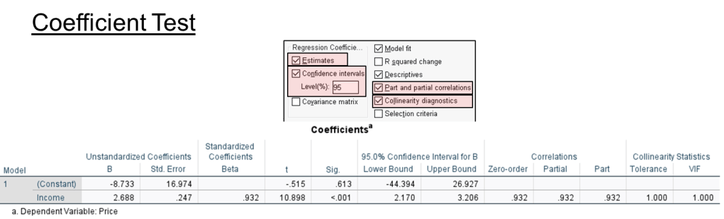
Step 11. Coefficient test result.
To form regression equation
price = -8.733 + 2.688 (income)
Income variable is part of the equation because its sig < 0..05.
Correlation
Zero-order = correlation between 2 variable (independent and dependent), without controlling for other variable
Partial = correlation between independent and dependent controlling for other variable impact on both dependent and independent variable.
Part = balance of zero-order minus partial.
Collinearity test result
VIF value < 10, no multicollinearity.
If more than 1 independent variable, we need to divide coefficient beta to obtain effect ratio. Eg.
Income = 1.001
Age = -0.093
abs(1.001) / abs(-0.093) = 10.763 ~ 11.
income has 11 times more effect on price than age.

Leave a comment