Tutorial 4

Question 1

The table below shows the result after fitting a time series data by an ARIMA model.

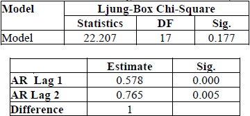
(a) Write the ARIMA model equation based on the results above.

(b) Represent the ARIMA model in ARIMA (p, d, q).

(c) Is the ARIMA model adequate? Justify your answers.

(d) Are all the AR coefficients in the ARIMA model significant at α = 0.05?

Example Answer

---

Question 2

The table below shows the result after fitting by ARIMA model.

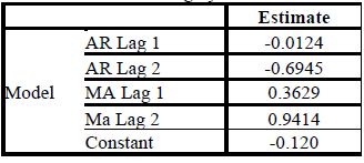
Write the model equation based on the parameter estimate values in the table.

Example Answer

ARIMA(2, 0, 2)

Y_t = -0.12 – 0.0124Y_t-1 – 0.6945Y_t-2 + ε_t + 0.3629ε_t-1 + 0.9414ε_t-2

---

Question 3

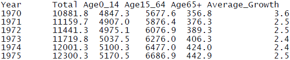
You are required to analyse the population data in Malaysia from 1970 to 2019 using R. You may download the data by clicking the link given: https://www.dosm.gov.my/v1/index.php?r=column/ctimeseries&menu_id=bnk3bk0wTTkxOXVHaVg3SUFDMlBUUT09

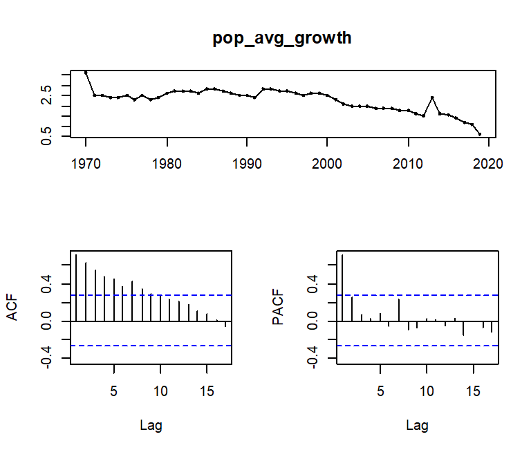
(a) Obtain a time series plot, ACF and PACF plots for Average Growth. Based on the plots, tentatively identify 3 appropriate ARIMA models for the data. You may require to use differencing if the data is not stationary. Apply appropriate statistical test to support your finding.

(b) Fit the 3 ARIMA models in part (a) to the data. Interpret your results.

(c) Perform diagnostic check the determine the adequacy of your fitted ARIMA models in part (b).

(d) After a satisfactory model has been found, forecast the average growth of population for the next 5 years. How does your forecast differ from the naïve forecast.

Example Answer

(a)

#Prepare data
Population_Malaysia <- read_excel("C:/Population_Malaysia.xlsx")
pop_avg_growth <- ts(Population_Malaysia$`Average annual population growth rate (%)`,
                     start=1970)

#Timeseries plot, ACF & PACF
library(forecast)
tsdisplay(pop_avg_growth)

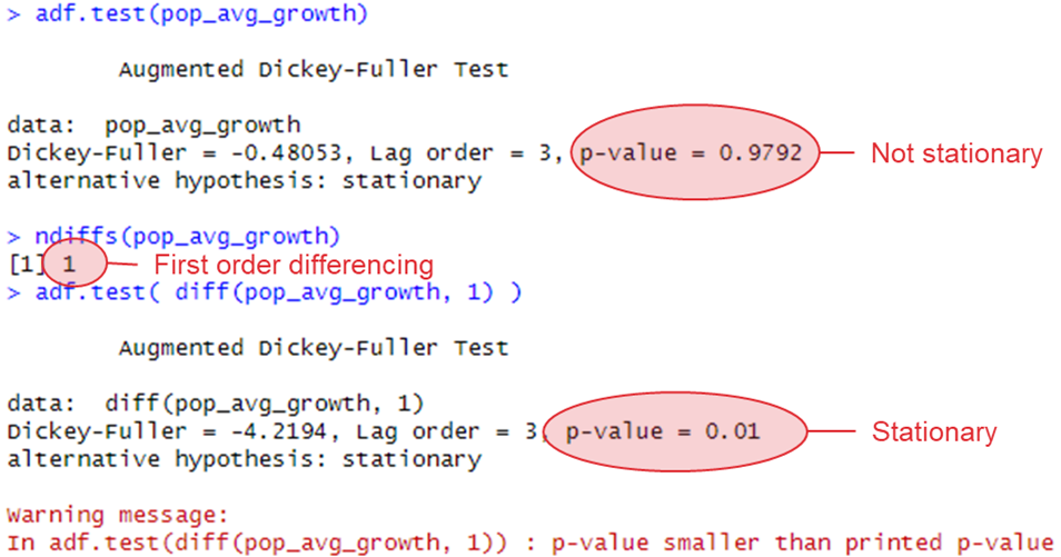
#Check data if stationary
library(tseries)
adf.test(pop_avg_growth)

#Check order of differencing needed
ndiffs(pop_avg_growth)

#Check data if stationary
adf.test( diff(pop_avg_growth, 1) )

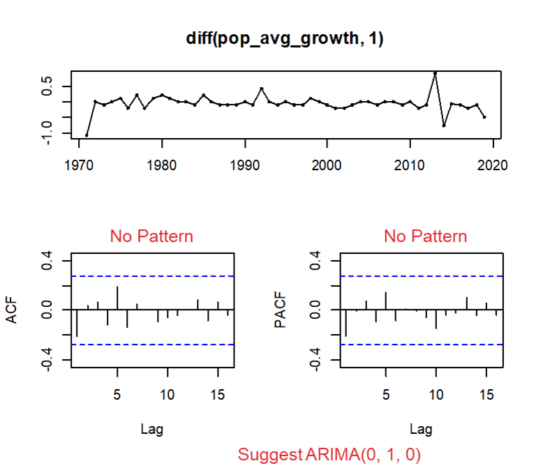
#Timeseries plot, ACF & PACF
tsdisplay( diff(pop_avg_growth, 1) )

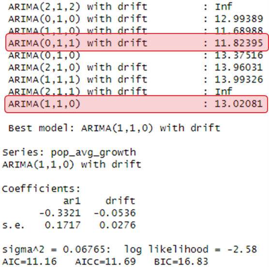
#Ultilized auto.arima for ARIMA hyperparameter suggestion
auto.arima(pop_avg_growth, trace=TRUE)
# pick ARIMA(0,1,0)                    : 13.37516
# pick ARIMA(1,1,0)                    : 13.02081 (stationary plot base on graph, PACF drop significant after lag 1, although below dotted line)
# pick ARIMA(0,1,1) with drift         : 11.82395 (Because it is the lowest in drift, apart from elected combination)

Result:

---

(b)

pop_arima_010 <- Arima(pop_avg_growth, order=c(0,1,0))
pop_arima_110 <- Arima(pop_avg_growth, order=c(1,1,0))
pop_arima_011 <- Arima(pop_avg_growth, order=c(0,1,1))

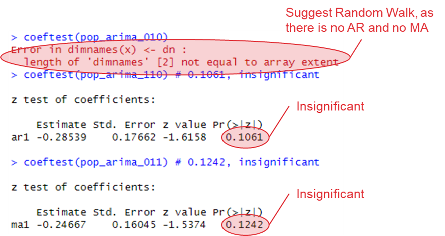
library(lmtest)
# use this function to get Pr(>|z|)
coeftest(pop_arima_010) # error, random walk
coeftest(pop_arima_110) # 0.1061, insignificant
coeftest(pop_arima_011) # 0.1242, insignificant

Result:

---

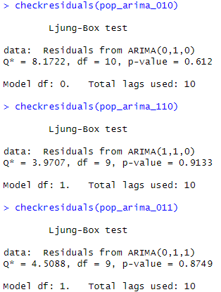
(c)

checkresiduals(pop_arima_010)
checkresiduals(pop_arima_110)
checkresiduals(pop_arima_011)

Result:

---

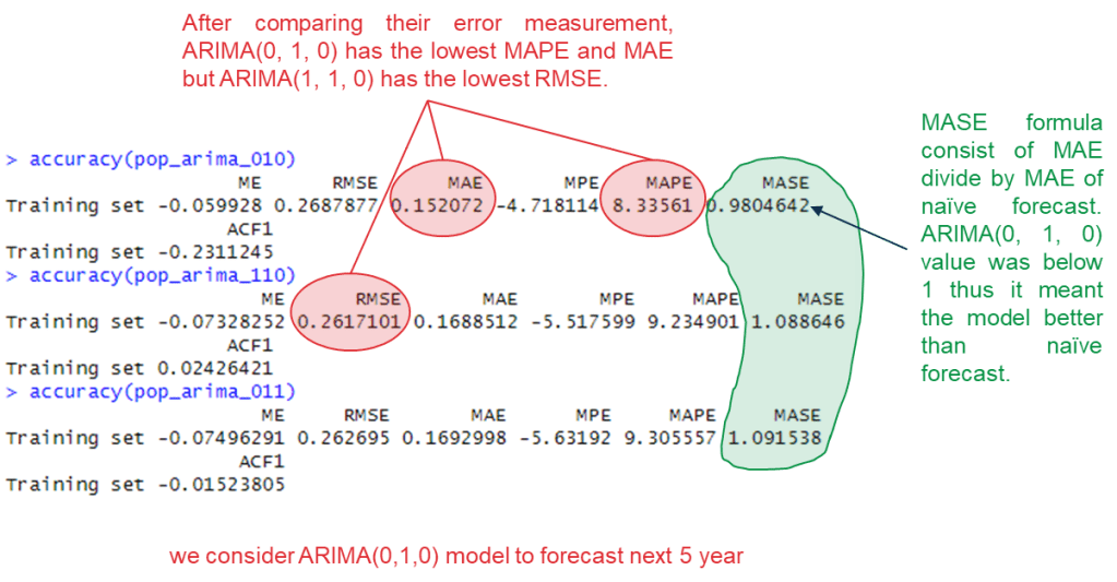
(d)

accuracy(pop_arima_010)
accuracy(pop_arima_110)
accuracy(pop_arima_011)

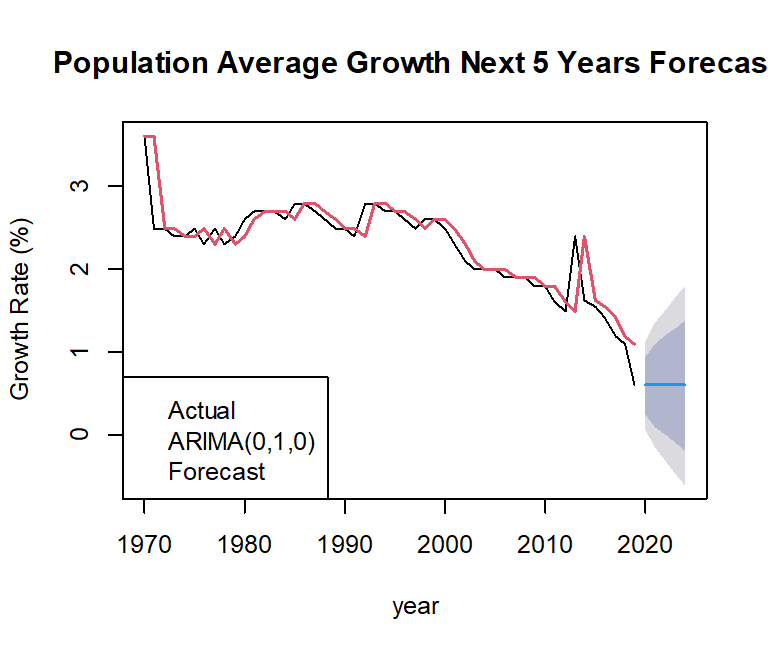
forecast_pop <- forecast(pop_arima_010, h=5)
plot(forecast_pop,
     main="Population Average Growth Next 5 Years Forecast",
     xlab="year",
     ylab="Growth Rate (%)")
lines(forecast_pop$fitted,
      col = 2,
      lwd=2)
legend("bottomleft",
       c("Actual", "ARIMA(0,1,0)","Forecast"),
       col=c(1:2, "blue"),
       )

Result:

---

Question 4

The following output is obtained after performing 1st seasonal differencing.

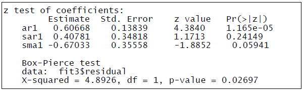
Write the model equation and interpret the results at α = 0.05.

Example Answer

ARIMA(1, 0, 0)(1, 1, 1)_s

Y_t = 0.60668Y_t-1 + 1.40781Y_t-s – 0.65522Y_t-1-s – 0.40781Y_t-2s + 0.24741Y_t-1-2s + ε_t – 0.67033ε_t-s

---

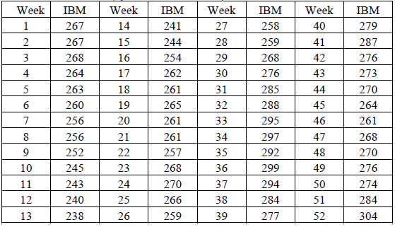
Question 5

The data below are weekly prices for IBM stock

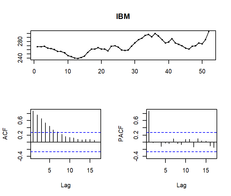
(a) Using a computer program for ARIMA modeling, obtain a plot of the data, the sample autocorrelations, and the sample partial autocorrelations. Use the information to tentatively identify an appropriate ARIMA model for the series.

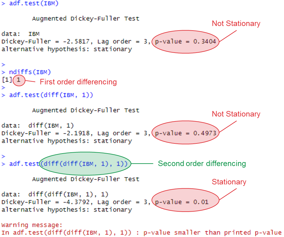
(b) Is the IBM series stationary? What correction would you recommend if the series is non-stationary?

(c) Fit an ARIMA model to the IBM series. Interpret the results.

(d) Perform the diagnostic check to determine the adequacy of your fitted model.

(e) After a satisfactory model has been found, forecast the IBM stock price for the first week of January of the next year. How does your forecast differ from the naïve forecast, which says that the forecast for the first week of January is the price for the last week in December (current price)?

Example Answer

(a)

IBM <- ts(T4.Q4$IBM)
tsdisplay(IBM)

Result:

---

(b)

adf.test(IBM) 

ndiffs(IBM) 

adf.test(diff(IBM, 1)) 

adf.test(diff(diff(IBM, 1), 1)) 

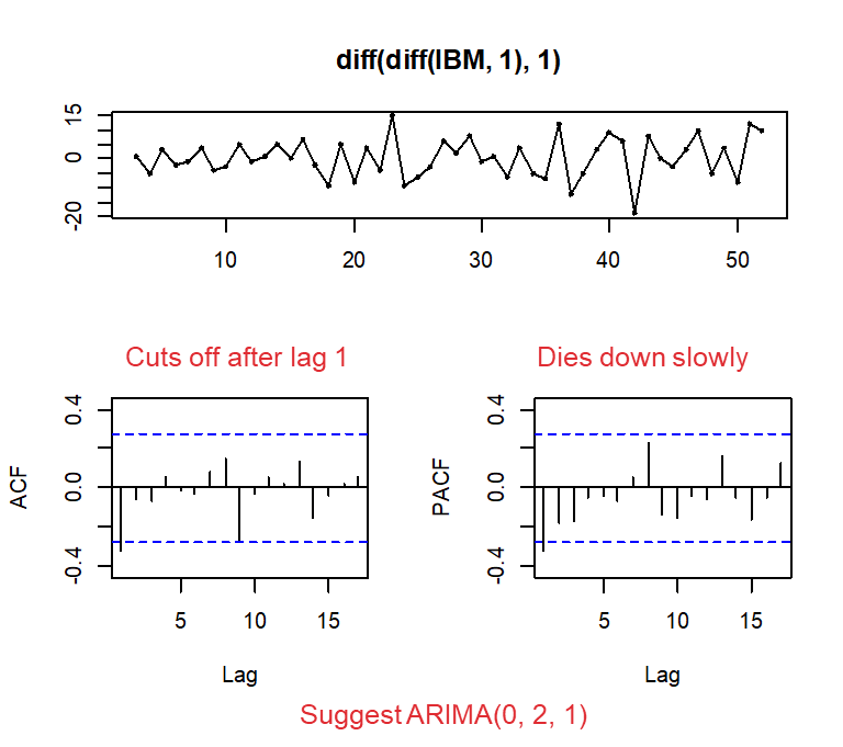
tsdisplay( diff(diff(IBM, 1), 1) )

auto.arima(IBM, trace=TRUE)

Result:

---

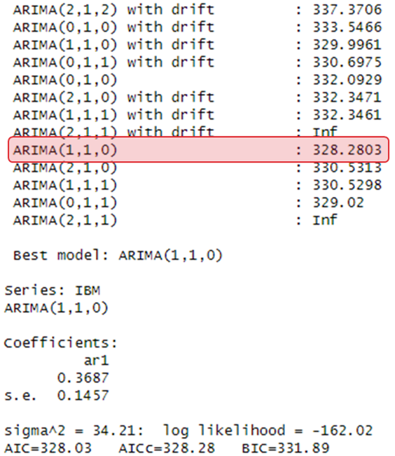
(c)

IBM_arima_021 <- Arima(IBM, order=c(0,2,1))
IBM_arima_110 <- Arima(IBM, order=c(1,1,0))

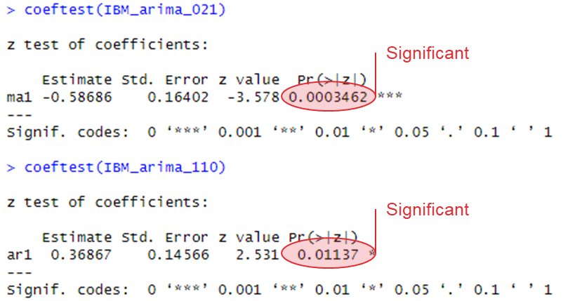
coeftest(IBM_arima_021)
coeftest(IBM_arima_110)

Result:

---

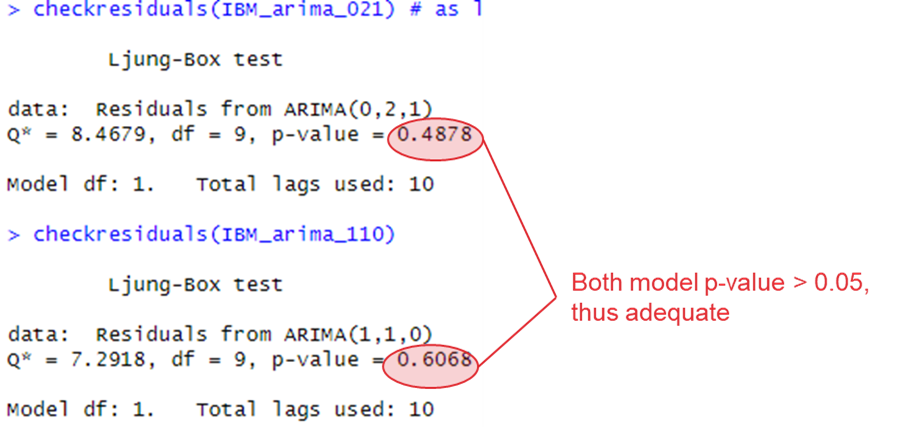
(d)

checkresiduals(IBM_arima_021)
checkresiduals(IBM_arima_110)

Result:

---

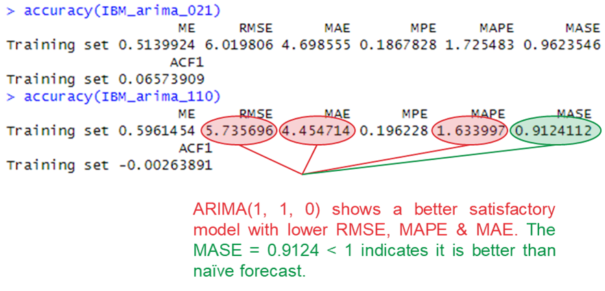
(e)

accuracy(IBM_arima_021)
accuracy(IBM_arima_110)

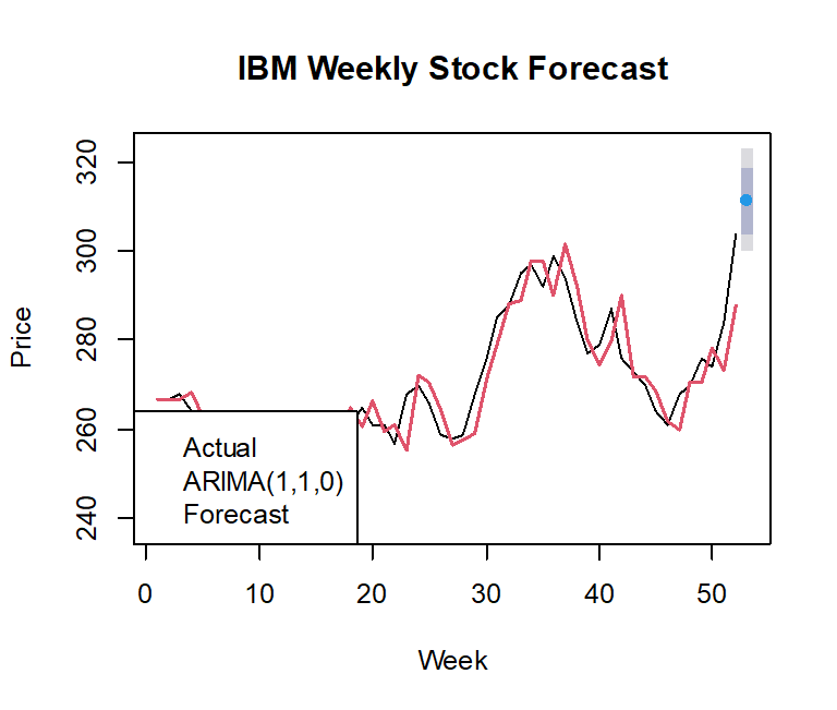
forecast_IBM <- forecast(IBM_arima_110, h=1)

plot(forecast_IBM,
     main="IBM Weekly Stock Forecast",
     xlab="Week",
     ylab="Price")
lines(forecast_IBM$fitted,
      col = 2,
      lwd=2)
legend("bottomleft",
       c("Actual", "ARIMA(1,1,0)","Forecast"),
       col=c(1:2, "blue"),
)

Result:

---

Question 6

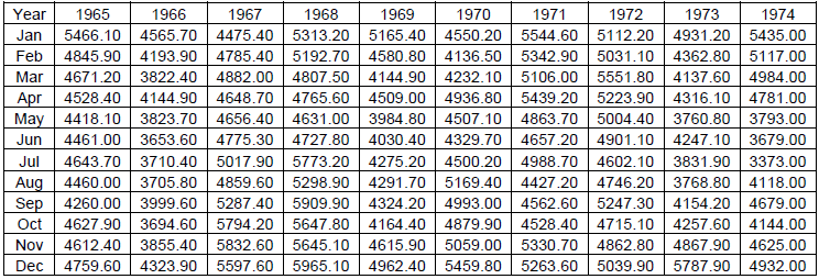
Table below contains a time series for monthly values of average weekly total investments at large New York City Banks, 1965 – 1974 (millions of dollars). Using a computer program for SARIMA modeling, obtain a plot of the data, the sample autocorrelations, and the sample partial autocorrelations. Develop an appropriate SARIMA model, and generate forecasts for the first three months of the year 1975.

Example Answer

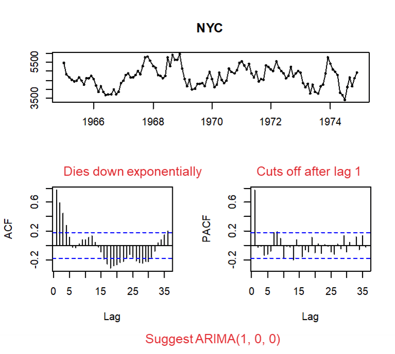
NYC <- ts(T4.Q6$Investment, start=1965, frequency=12)
tsdisplay(NYC)

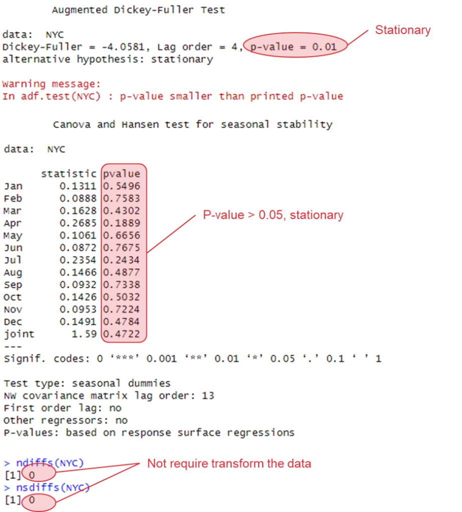
adf.test(NYC)

library(uroot)
ch.test(NYC)

ndiffs(NYC)
nsdiffs(NYC)

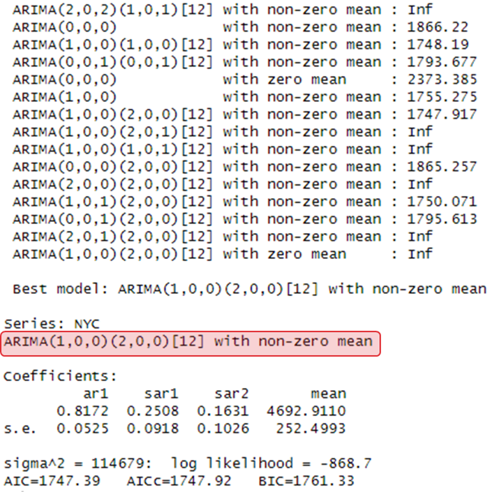
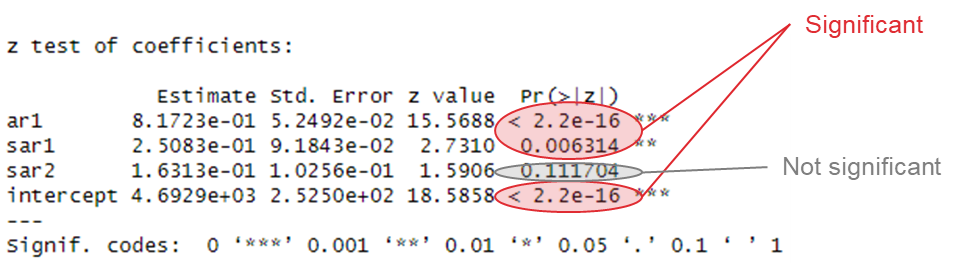
auto.arima(NYC, trace=TRUE)

NYC_arima_100 <- Arima(NYC, order=c(1,0,0), seasonal=c(2,0,0))


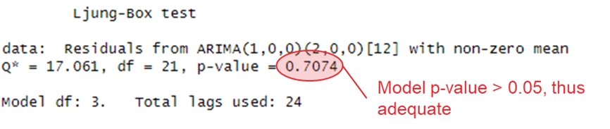
checkresiduals(NYC_arima_100)

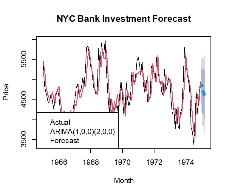
forecast_NYC <- forecast(NYC_arima_100, h=3)

plot(forecast_NYC,
     main="NYC Bank Investment Forecast",
     xlab="Month",
     ylab="Price")
lines(forecast_NYC$fitted,
      col = 2,
      lwd=2)
legend("bottomleft",
       c("Actual", "ARIMA(1,0,0)(2,0,0)","Forecast"),
       col=c(1:2, "blue"),
)

Result:

---