
Box Jenkins Methodology (Recap)
Split the below data into training (80%) and testing data (20%). Analyse the training data and formulate the model equation for the ARIMA model you chosen:
Then, compute the accuracy of the model in the testing data. Check the residuals and test whether the model you chosen is satisfactory.
Sales
Import data.
Sales <- read.csv("C:/sales.dat", sep="")
Sales = ts(Sales, start=2007, frequency=4)
Split Train/Test.
train_sales <- Sales[1:(0.8 * length(Sales))]
test_sales <- Sales[-c(1:(0.8 * length(Sales)))]
Check stationary and ARIMA hyperparameter.
library(forecast)
tsdisplay(train_sales, lag.max = 28)
Result:
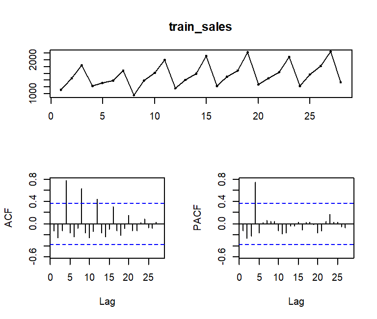
Explanation:
ACF (MA) show seasonal dies down slowly (not stationary)
PACF (AR) show cuts off at lag 1
Check stationary again with adh test.
library(tseries)
ndiffs(train_sales)
nsdiffs(train_sales)
Result:

Explanation:
Variable was in list data type, not in time series data type.
Convert variable into time series data type.
train_sales <- ts(train_sales, start=2007, frequency=4)
test_sales <- ts(test_sales, start=2014, frequency=4)
Check stationary again with adh test. (with proper data type)
ndiffs(train_sales)
nsdiffs(train_sales)
Result:

Explanation:
Result show differencing action is needed.
Stationary check after differencing.
adf.test( diff(train_sales, 4) )
library(uroot)
ch.test( diff(train_sales, 4) )
Result:

Explanation:
ch.test does not show any “*”, meaning seasonal is now stationary.
Check ACF & PACF plot for ARIMA hyperparameter.
tsdisplay(diff(train_sales, 4), lag.max = 28)Result:
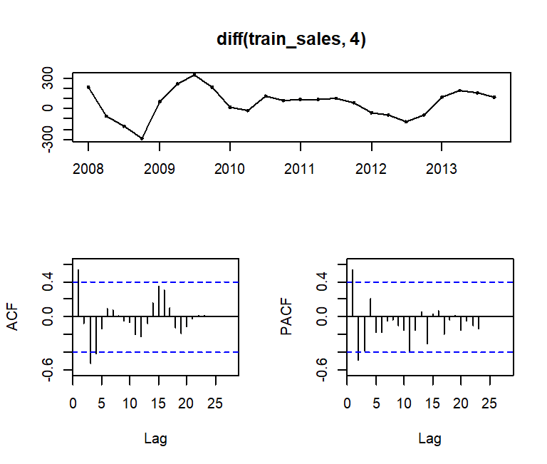
Explanation:
ACF show cuts off, and seasonal ACF shows cuts off as well.
PACF show dies down exponentially, seasonal show no pattern.
This suggested
ARIMA(0, 0, 1)(0, 1, 1)4
Train an ARIMA model.
sales_arima_001_011 <- Arima(train_sales,
                             order=c(0,0,1),
                             seasonal=c(0,1,1))
Check if model adequate.
checkresiduals(sales_arima_001_011)Result:

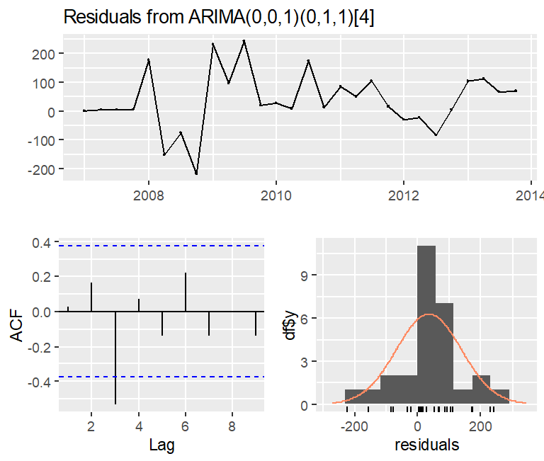
Explanation:
p-value = 0.01 < 0.05, this show the model is not adequate.
Use auto.arima to seek for new hyperparameter.
auto.arima(train_sales, trace=TRUE)Result:

Explanation:
Although ARIMA(0, 0, 2)(0, 1, 1) with drift is highly suggested, the syllabus does not include drift model. thus only consider those without drift wording, ARIMA(0, 0, 2)(0, 1, 1).
Train a new model and check adequate.
sales_arima_002_011 <- Arima(train_sales,
                             order=c(0,0,2),
                             seasonal=c(0,1,1))
checkresiduals(sales_arima_002_011)
Result:
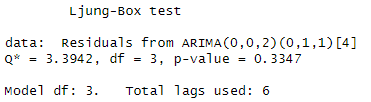
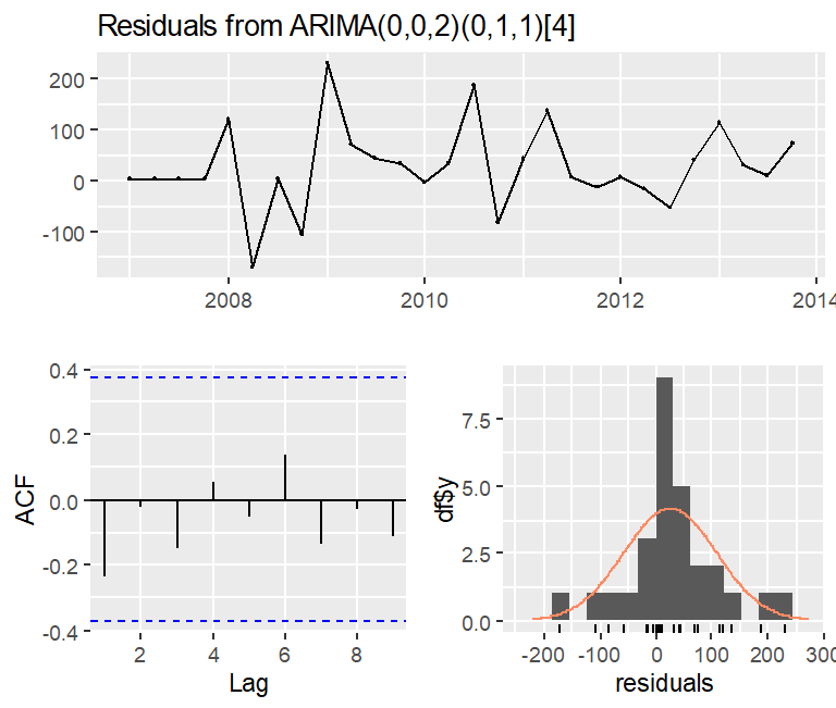
Explanation:
p-value = 0.3347 > 0.05, this show the model is adequate.
Generate forecast value.
forecast_sales_arima_002_011 <- forecast(sales_arima_002_011,
                                         h=length(test_sales))
Check accuracy with Test subset.
accuracy(forecast_sales_arima_002_011,
         test_sales)
Result:
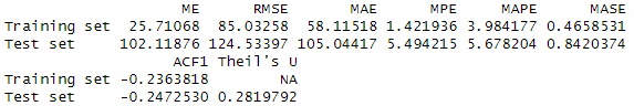
ps. The formula will be:
Yt = Yt-4 + εt + 0.98507εt-1 + 0.78824εt-2 – 0.34295εt-4
the symbol value derive from
coeftest(sales_arima_002_011)Result:
Beer Production
#Prepare data
USABeerproduction <- read_csv("USABeerproduction.csv")
beer = USABeerproduction$beerproductionusa
beer = ts(beer, start=1970, frequency=12)

#Split Train/Test
train_beer <- beer[1:(0.8 * length(beer))]
test_beer <- beer[-c(1:(0.8 * length(beer)))]

#Check stationary, arima hyperparameter
tsdisplay(train_beer, lag.max=60)

#Check stationary
ndiffs(train_beer)
nsdiffs(train_beer)

#Set the datatype into timeseries
train_beer <- ts(train_beer, start=1970, frequency=12)

#Check stationary
ndiffs(train_beer)
nsdiffs(train_beer)

#Check stationary after differencing
adf.test(diff(diff(train_beer, 1), 12))
ch.test(diff(diff(train_beer, 1), 12))

#Check arima hyperparameter
tsdisplay(diff(diff(train_beer, 1), 12), lag.max=60)

#Train an ARIMA model
beer_arima_011_010 <- Arima(train_beer, order=c(0,1,1), seasonal=c(0,1,0))

#Check different hyperparameter importancy
coeftest(beer_arima_011_010)

#Check model adequate
checkresiduals(beer_arima_011_010)

#Predict next h value
forecast_beer_arima_011_010 <- forecast(beer_arima_011_010, h=length(test_beer))

#Check forecast value and test subset metrics
accuracy(forecast_beer_arima_011_010, test_beer)

#Check any better hyperparameter
auto.arima(train_beer)

#Train next ARIMA model
beer_arima_100_012 <- Arima(train_beer, order=c(1,0,0), seasonal=c(0,1,2))

#Check model adequate
checkresiduals(beer_arima_100_012)

#Predict next h value
forecast_beer_arima_100_012 <- forecast(beer_arima_100_012, h=length(test_beer))

#Check forecast value and test subset metrics
accuracy(forecast_beer_arima_100_012, test_beer)
Result:

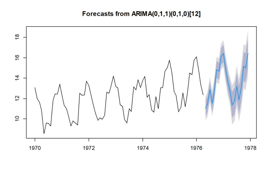
plot(forecast_beer_arima_011_010)Result:

Leave a comment