Box Jenkins Methodology

A step by step process to identify and fitting ARIMA model hyperparameter; as the model itself has 3 main component:

1. Autoregression [AR]
2. Differencing aka integrated [I]
3. Moving average [MA]

In R, the model will be wrote as ARIMA (data, order=c(p aka [AR], d aka [I], q aka [MA])).

ARIMA rely on stationary data; throw back to Day 56, there are 4 criteria (constant mean, constant variance, constant covariance & auto correlation) to justify the data is stationary.

As auto correlation is one of the main criteria and can be visualized by ACF & PACF plot, there are a need to understand what kind of ACF/PACF we seeking for.

---

Step 1. Identify stationary

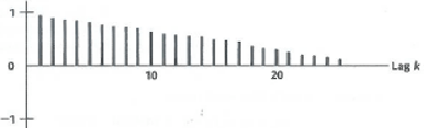
Stationary

Damped exponential dying down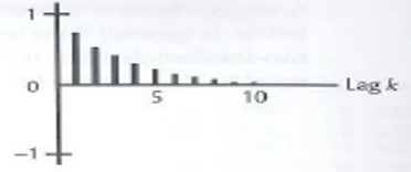	Damped sine-wave dying down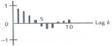
Damped exponential dying down with oscillation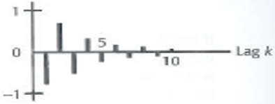	Cut off after lag 2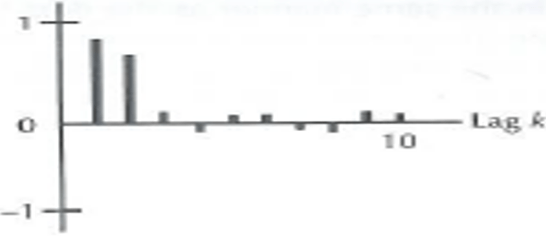 The point where cut off happen will be feed-ed into the ARIMA hyperparameter.

Non Stationary

---

R

quakes <- ts(Earthquakes)

library(forecast)
tsdisplay(quakes)

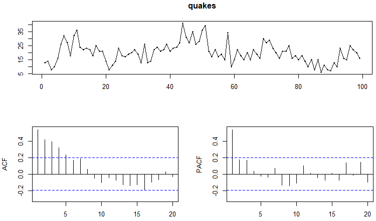
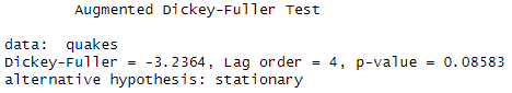
Note that PACF show stationary but ACF does not.; and in this case, PACF > ACF (means that PACF at higher order). Before deep dive into ordering, first we need to make sure the time series are stationary. Check using Augmented Dickey–Fuller Test function.

library(tseries)
adf.test(quakes)

Another checking can be done using

ndiffs(quakes)

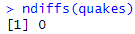
Boom! ndiffs show the quakes time series is stationary but adh test show otherwise. Here I keep a suspense later to be discuss.

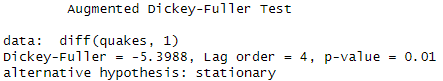
Since the quakes time series is not stationary confirmed by both test, we need to “station” it.

adf.test( diff(quakes, 1) )

and we can finally check both ACF and PACF.

tsdisplay( diff(quakes, 1) )

Now lets conclude step 1. ACF cut off after lag 1. PACF dies down exponentially.

---

Step 2. Fill-up hyperparameter

[AR]	[I]	[MA]
0	1	1

How to come out with this setting?

First, lets talk about middle [I] equal to 1. The reason this is 1 is because [I] means differencing, we had perform diff = 1 before we generate the chart.

Second why [AR] = 0 and [MA] = 1? Remember the ordering? Both ACF and PACF chart must be compare, cut off is the dominant, like Ace in poker. ACF had shown dominant and following rule relate how [MA] equal to 1.

so now ACF cut off at 1, equal to [MA](1) whereas it dominant to PACF, so [AR](0). Let’s train our model using the hyperparameter we discover.

quakes_arima_011 <- Arima(quakes, order=c(0,1,1))

---

Step 3. Setup the alien language

So….what the hell is this? Say for example, we are given some value relevant to the symbol above, we can calculate the forecast value! Don’t ask me why someone will do that, i’m speechless but this step actual help to conclude why AR is call autoregression, MA is call moving average and I is call integrated.

BY_t = Y_t-1 aka B^kY_t = Y_t-k aka (1 – B)^dY_t

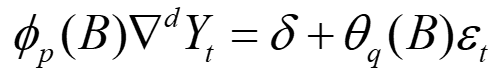
Before going in, there are something call Backshift operator. I would assume this is the soul to the alien language. It is meant to expanding the formula.

ϕp (B)	∇d	Yt	=	δ	+θq (B)	εt
This is the [AR] part, where it will be expanding base on the hyperparameter number	This is the [I] part.	Forecast value		A constant value	This is the [MA] part.	An error value
1 – ϕ1B – ϕ2B2	(1-B)d				1 + θ1B + θ2B2

Notice both AR and MA has B inside the formula? Backshift operator will be replacing the B so that the whole formula would be remaining Y (depending exact value or error (actual – forecast).

Now, from above quakes time series, we know the ARIMA going to be AR(0)I(1)MA(1), how can we formulate it?

Since AR equal 0 (zero), first column can be remove; Leaving the formula like

∇^d Y_t = δ + θ_q(B) ε_t

[I] equal to 1, ∇^d will become (1-B)^d . Leaving the formula like

(1 – B)¹ Y_t = δ + θ_q(B) ε_t

Using the backshift operator on B¹ Y_t the result will be Y_t-1. Leaving the formula like

Y_t – Y_t-1 = δ + θ_q(B) ε_t

In the quakes time series, there are no constant value. ps. I suspect constant value meaning the constant mean after diff(1), cause the data were at 0 constant mean.

Leaving the formula like

Y_t – Y_t-1 = θ_q(B) ε_t

The number of [MA] will be use here, and since [MA] was 1, θ_q(B) will be 1 + θ₁B. Same case for [MA] = 2, it will be

1 + θ₁B + θ₂B². Leaving the formula like

Y_t – Y_t-1 = (1 + θ₁B) ε_t

We need to multiply the epsilon ε_t into the [MA]. Leaving the formula like

Y_t – Y_t-1 = ε_t + θ₁Bε_t

Remove the B as B equal to B¹, look into backshift operator. Leaving the formula like

Y_t – Y_t-1 = ε_t + θ₁ε_t-1

Move – Y_t-1 to the right side. Leaving the formula like

Y_t = ε_t + θ₁ε_t-1 + Y_t-1

Now likes find θ

summary(quakes_arima_011)

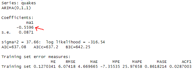
Leaving the formula like

Y_t = ε_t + ( -0.5596 ε_t-1 ) + Y_t-1

So what’s next? Replace everything and use the formula to forecast!

ps. Since [MA] is using the delta between actual and forecast, it could consider average? And [AR] is using the actual value, thus the name regression.

---

Step 3. Compare with Auto.arima (_{^{Actual step, earlier step is meant for class test.}})

Remember earlier in ndiffs test, we saw it suggest that the data was stationary? Auto.arima function uses that to prepare suggestion for us.

auto.arima(quakes, trace=TRUE)

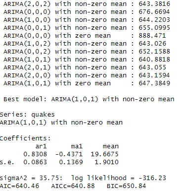
Auto.arima is a tool that compute possible hyperparameter that best predict the quakes time series. Earlier, we had been using ARIMA(0, 1, 1) and now lets train another model with ARIMA(1, 0, 1).

quakes_arima_101 <- Arima(quakes, order=c(1,0,1))

ps. Remember earlier PACF dies down exponentially? this would also means that the lag could by ranging anything from 0-2 (after lag the, the value was within the dotted line).

---

Step 4. Compare RMSE between model

Since we had 2 model, let’s compare side by side.

summary(quakes_arima_011)
summary(quakes_arima_101)

In this case, we saw that auto.arima actually suggested a better RMSE & MAE model. How about the residual?

checkresiduals(quakes_arima_011)
checkresiduals(quakes_arima_101)

Result:

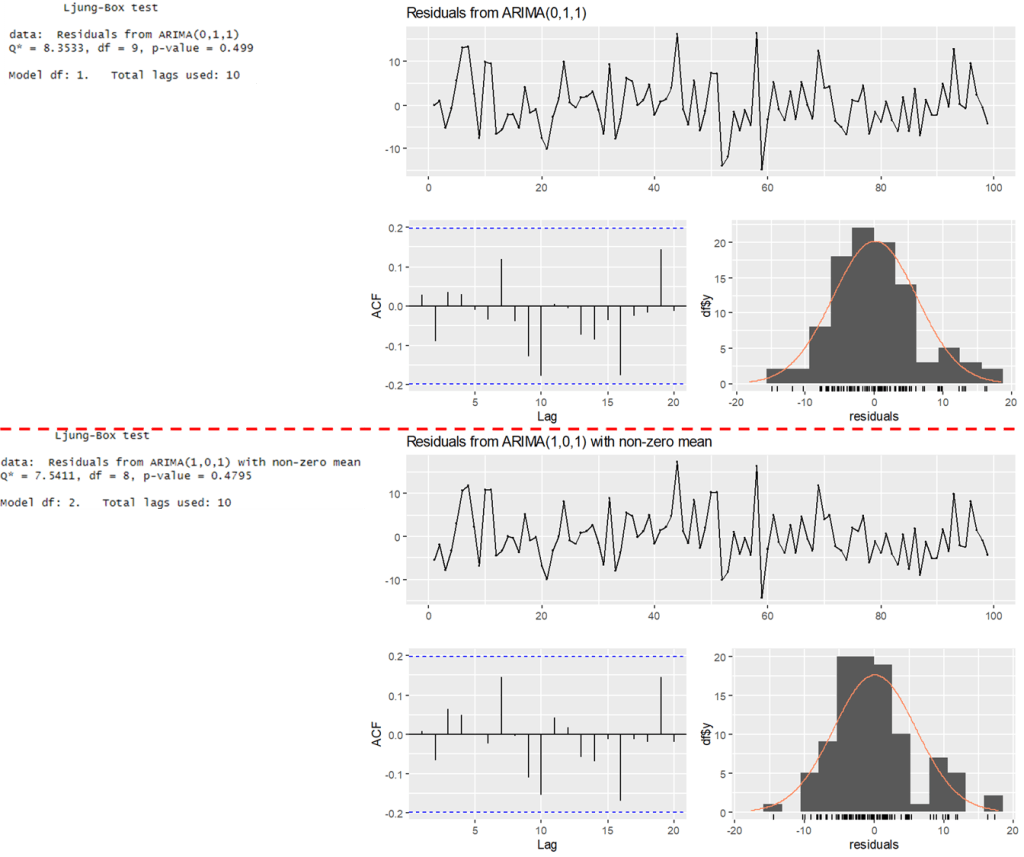
As both model p-value are > 0.05, the models are adequate.

However, we are unable to tell the does the model facing any overfitting issue. Data Partitioning into Train/Test would be useful to tell us the result. Lets copy some of the code from yesterday.

train_quakes <- quakes[ 1 : ( 0.8 * length( quakes ) ) ]
test_quakes <- quakes[ -c( 1 : ( 0.8 * length( quakes ) ) ) ]

and create the same model using training dataset.

quakes_train_arima_011 <- Arima(train_quakes, order=c(0,1,1))
quakes_train_arima_101 <- Arima(train_quakes, order=c(1,0,1))

make prediction with test dataset length.

quakes_forecast_arima_011 <- forecast(quakes_train_arima_011, h=length(test_quakes))
quakes_forecast_arima_101 <- forecast(quakes_train_arima_101, h=length(test_quakes))

check the accuracy for both model

accuracy(quakes_forecast_arima_011, test_quakes)

accuracy(quakes_forecast_arima_101, test_quakes)

Well, we can see that both of the model was are not overfitted as the predicted data does not vary significantly to test dataset. Auto.arima model perform slightly worst that our model in comparison of overfitting.

There are also extra step to compute the formula, say if we wish to further finetune our model performance, we can check into coeftest

library(lmtest)
coeftest(quakes_arima_011)

What does it mean here? Say for example cases like below, [SMA](1) does not have asterisk that signal p-value < 0.05, in this case, we can drop it from the Arima hyperparameter.

---

---

---

SARIMA

Again, let’s dive into the alien language.

The capital [S] actually mean to introduce seasonality into the model. Recall from Day 58? Both Multi-Linear Regression and Winter Holt’s Exponential Smoothing introduce additional hyperparameter to represent seasonal pattern. Same case here.

Question 1

Example Answer

1. φ_p(B) Φ_P(B^S) ∇_S^D ∇^d Y_t = δ + θ_q(B) Θ_Q(B^S) ε_t
2. φ_p(B) Y_t = δ + Θ_Q(B^S) ε_t :==: remove all un-needed component like [SAR], [SI], [I] and [MA].
3. (1 – φ_p) Y_t = δ + (1 + Θ_Q) ε_t :==: remove B and expand the formula
4. Y_t – φ_pY_t-1 = δ + ε_t + Θ_Qε_t-4 :==: remove bracket and fill back B = -1 for normal, and B = -4 for seasonality.
5. Y_t = δ + ε_t + Θ_Qε_t-4 + φ_pY_t-1 :==: move everything to the right.
6. Y_t = 1630.9404 + ε_t + 0.8037ε_t-4 + 0.1051Y_t-1 :==: replace the symbol with value above.

Question 2

Example Answer

1. we saw [AR](1) [MA](1), [SMA](1), other component not found and assume null aka ARIMA(1, 0, 1)(0, 0, 1)
2. φ_p(B) Φ_P(B^S) ∇_S^D ∇^d Y_t = δ + θ_q(B) Θ_Q(B^S) ε_t
3. φ_p(B) Y_t = θ_q(B) Θ_Q(B^S) ε_t :==: remove all un-needed component like constant mean, [SAR], seasonal [I] and [I].
4. Y_t – φ_pY_t-1 = (1 + θ_q(B))(1 + Θ_Q(B^S)) ε_t :==: expand B.
5. Y_t – φ_pY_t-1 = 1 + θ_q(B) + Θ_Q(B^S) + θ_qΘ_Q(B^{1 + S}) ε_t
6. Y_t – φ_pY_t-1 = ε_t + θ_qε_t-1 + Θ_Qε_t-s + θ_qΘ_Qε_t-1-s
7. Y_t = ε_t + θ_qε_t-1 + Θ_Qε_t-s + θ_qΘ_Qε_t-1-s + φ_pY_t-1 :==: move everything to the right.
8. Y_t = ε_t + 0.23030ε_t-1 – 0.21569ε_t-s – 0.04967ε_t-1-s + 0.51225Y_t-1 :==: replace the symbol with value above.

Say why we looking into SARIMA? It is because sometime ACF & PACF plot show seasonality.