
Recap. Differencing vs smoothing = differencing is about removing trend from time series, by “station” the data back to its mean; smoothing in the other hand focus on removing irregular signal to uncover pattern (trend & seasonality).
Tutorial 2
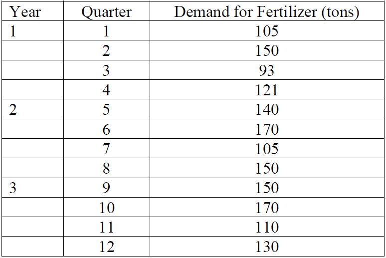
Question 1
(a) Compute a three-quarter moving average forecast for quarters 4 through 13.
(b) Compute a five-quarter moving average forecast for quarters 6 through 13.
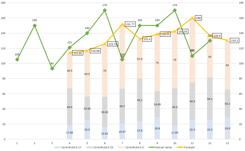
(c) Compute a weighted three-quarter moving average forecast using weights of 0.50, 0.33, and 0.17 for the most recent, next recent and most distant data respectively.
Example Answer
(a)

(b)

Tips. Remember to check predicted value are correctly using last n value in the formula.

(c)

Tips. WMA rely on “weight”.
Question 2
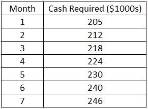
(a) Use 2-period exponential moving average to forecast cash requirements in August.
(b) Use 3-period weighted moving average to forecast cash requirements in August.
(c) Use simple exponential smoothing method with α = 0.4 to forecast cash requirements in August.
(d) Use Holts method with α = 0.6 and β = 0.4 to forecast cash requirements for the next two months.
Example Answer
(a) step 1

(a) step 2

(b)

(c)

(d)

Question 3
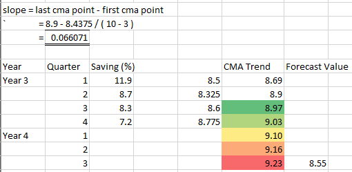
The following data describes personal savings as a percentage of earned income for a particular region of the country.
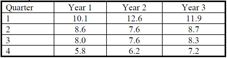
Express all the calculations in 2 decimal places.
(a) Use multiplicative model to seasonally adjust the above percentages.
(b) When does the region have the largest seasonal variation? How much it differs from the yearly average?
(c) Forecast the percentages savings for quarter 3 in Year 4.
Example Answer
(a)

(b)
Largest SV in quarter 1.
Different = 1.43 – 1 = 0.43
1 means every quarter donated 1 for 4 quarter, total 4
(c)
Question 4
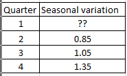
A multiplicative decomposition model is applied to a quarterly sales data from 2012 to 2016 and the seasonal variation for each quarter is shown below:
(a) Estimate the seasonal variation in Quarter 1.
(b) Based on the table above, when the sales have the lowest and largest seasonal variation respectively? How much they differ from the yearly average?
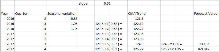
(c) Assume the last observed trend (CMA) is 121.50 and the average increment is 0.62, produce the forecast in Q3 and Q4, 2017 respectively.
Example Answer
(a)

(b)

(c)
Question 5
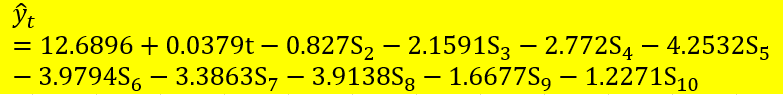
Answer the following question using dataset USABeerproduction.csv. The following output is obtained after fitted a regression model to the dataset (1970/1 – 1977/12).

Based on the above output, answer the following.
(a) Write down the regression model to estimate the beer production in the next period.
(b) Can we conclude that there is a trend component present in the series? Justify your answer.
(c) Can we conclude that there is a seasonal component present in the series? Justify your answer.
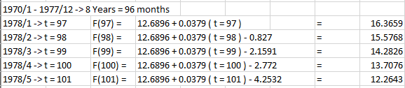
(d) Interpret the meaning of (-4.2532) for variable May in the regression model.
(e) Forecast the beer production from January to May, 1978.
Example Answer
(a)
(b)
Yes, there is a trend component present in the series. According to the output, the p-value of time is 0 that is less than 5% significant level. Therefore, reject H0. Thus, the slop parameter is significant.
(c)
Yes, there is a seasonal component present in the series. According to the output, majority of the p-values for the dummies are less than 5% significant level. Therefore, reject H0. Thus, the seasonal dummies are significant.
(d)
After accounting for the trend, beer production in May is average about 4.2532 unit less than December production. Note. why say 4.2532 less is because December is turning off all parameter, which means only using “12.6896 + 0.0379 x t”.
(e)
Question 6
Use the following forecasting model to forecast the beer production in the next 5 years using R.
(a) Exponential Smoothing
(b) Holts Method
(c) Holt Winters Method
(d) Decomposition Model (use STL function in R)
Example Answer
(a) SES
library(forecast)
beer <- read.csv("USABeerproduction.csv")
beer_ts = ts(beer$beerproductionusa,
             start=1970,
             frequency=12)

beer_ses <- ses(beer_ts,
                initial="simple",
                h=60)
plot(beer_ses,
     main="Beer Production Forecast for Next 5 Years",
     xlab="Year",
     ylab="Production")
lines(beer_ses$fitted,
      col=2,
      lwd=2)
legend("topleft",
       c("Actual", "SES", "Forecast"),
       col=c(1:2,"blue"),
       lwd=2,
       cex=0.7)
Result:

(b) Holt
beer_holt <- holt(beer_ts,
                  initial="simple",
                  h=60)
plot(beer_holt,
     main="Beer Production Forecast for Next 5 Years",
     xlab="Year",
     ylab="Production",
     ylim=c(0,30))
lines(beer_holt$fitted,
      col=2,
      lwd=2)
legend("topleft",
       c("Actual", "Holt", "Forecast"),
       col=c(1:2,"blue"),
       lwd=2,
       cex=0.7)
Result:

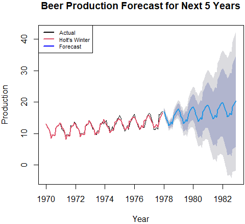
(c) Holt’s Winter
beer_hw <- hw(beer_ts,
              initial="simple",
              seasonal="additive",
              h=60)
plot(beer_hw,
     main="Beer Production Forecast for Next 5 Years",
     xlab="Year",
     ylab="Production")
lines(beer_hw$fitted,
      col=2,
      lwd=2)
legend("topleft",
       c("Actual", "Holt's Winter", "Forecast"),
       col=c(1:2,"blue"),
       lwd=2,
       cex=0.7)
Result:
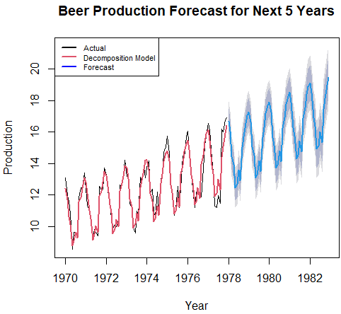
(d)
beer_stl <- stlf(beer_ts,
                 h=60)
plot(beer_stl,
     main="Beer Production Forecast for Next 5 Years",
     xlab="Year",
     ylab="Production")
lines(beer_stl$fitted,
      col=2,
      lwd=2)
legend("topleft",
       c("Actual", "Decomposition Model", "Forecast"),
       col=c(1:2,"blue"),
       lwd=2,
       cex=0.7)
Result:
Uploaded Answer

Leave a comment