
Smoothing Techniques
| Techniques | Focus on |
|---|---|
| Moving Average | Stationary / Irregular Component |
| Weighted Moving Average | |
| Exponential Moving Average | |
| Modified Moving Average | |
| Exponential Smoothing | |
| Holts Method | Trend Component |
| Linear / Quadratic / Exponential Trend | |
| Decomposition Model | Seasonal + Trend Component |
| Holts Winter Smoothing | |
| Dummy variable + Regression |
ps. Most of the time series forecast technique are under forecast/predicting, forecast line below actual value.
Moving Average
Develop N-week Moving Average forecasts for the below demand.
Excel
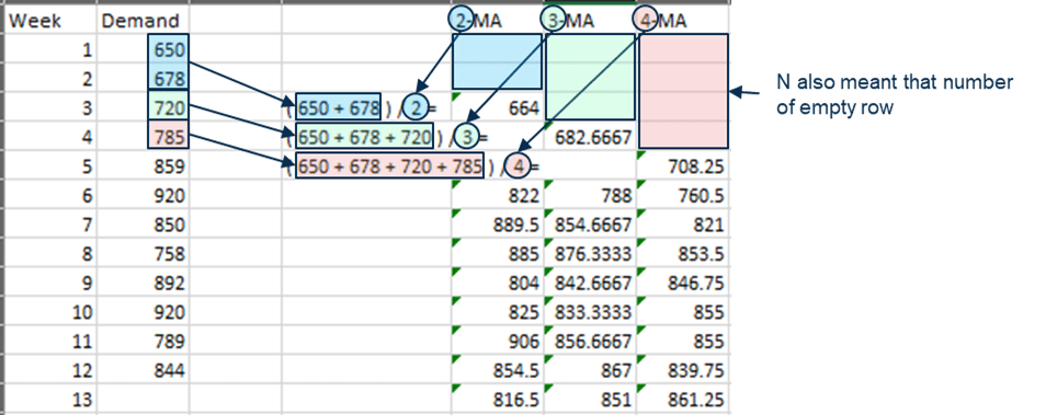
Result:
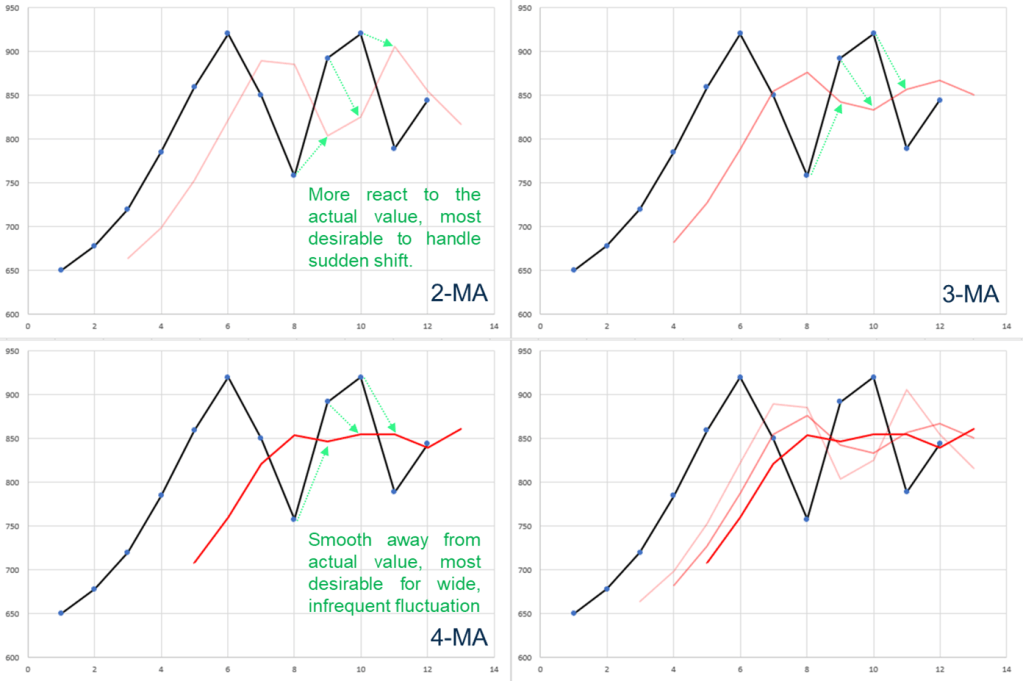
ps. MA heavily rely on data point, does not capture any historical trend.
R
SMA(data, n=2) → create simple moving average by 2.
SMA(c(650,678,720,785,859,920,850,758,892,920,789,844), n=2)Result:

plot(ts(c(650,678,720,785,859,920,850,758,892,920,789,844)))
lines(SMA(c(650,678,720,785,859,920,850,758,892,920,789,844), n=2),
      col=2,
      lwd=2)
Result:

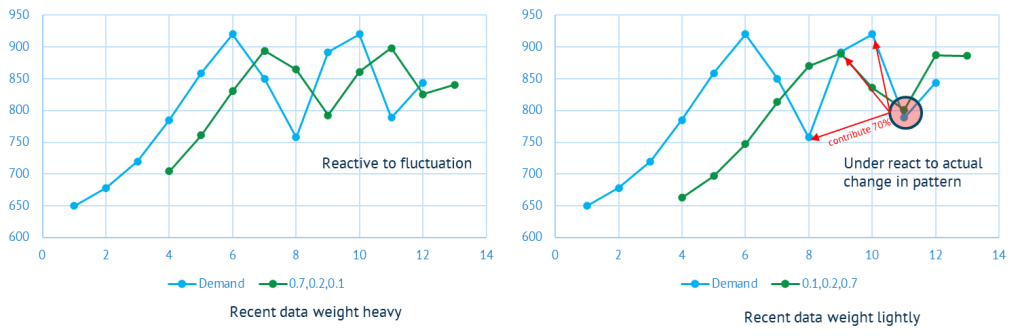
Weighted Moving Average
Develop 3-week Weighted Moving Average forecasts for the below demand, with weights = 0.7, 0.2 and 0.1 to the most recent, next recent and the most distant data.
Excel

Result:
R
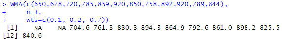
WMA(data, n=3,wts=c(0.1, 0,2, 0,7)) → create weighted moving average by 3; wts to configure weight.
WMA(c(650,678,720,785,859,920,850,758,892,920,789,844),
    n=3,
    wts=c(0.1, 0.2, 0.7))
Result:
plot(ts(c(650,678,720,785,859,920,850,758,892,920,789,844)))
lines(WMA(c(650,678,720,785,859,920,850,758,892,920,789,844),
          n=3,
          wts=c(0.1, 0.2, 0.7)),
      col=2,
      lwd=2)
Result:

Exponential Moving Average
Develop 3-week exponential forecasts for the below demand.
Excel

ps. first value normally perform SMA.
Result:

ps. EMA still rely on recent data point as it contribute the most; whereas smoothing factor were added to it.
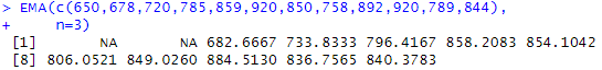
R
EMA(data, n=3) → create exponential moving average by 3.
EMA(c(650,678,720,785,859,920,850,758,892,920,789,844),
    n=3)
Result:
plot(ts(c(650,678,720,785,859,920,850,758,892,920,789,844)))
lines(EMA(c(650,678,720,785,859,920,850,758,892,920,789,844), n=3),
      col=2,
      lwd=2)
Result:

Modified Moving Average
Develop 3-week modified Moving Average forecasts for the below demand.

ps. Apparently MMA is depends to how you modified any MMA. In this case, it is modified from 3-EMA.
Exponential Smoothing (SES)
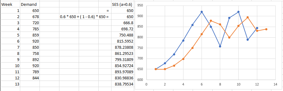
Excel
Determine exponential smoothing forecasts for periods 2-10 using a = 0.1 and a = 0.6, assuming F1 = D1
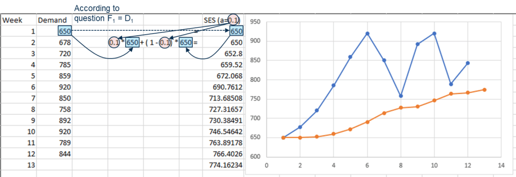
ps. Procedure for continually revising a forecast in the light of more recent experience, backward propagation. If alpha = 1, that means fully rely on previous value; aka naive forecast.
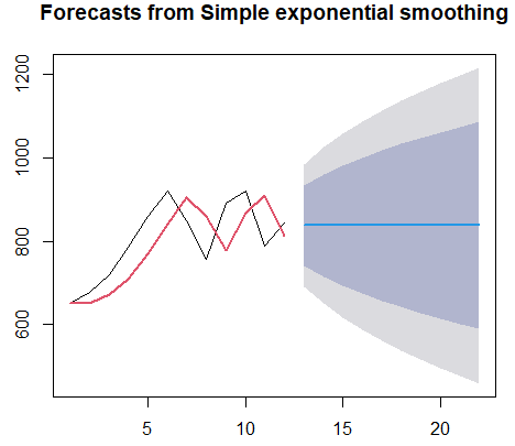
R
ses(data, initial=”simple”, h=number of forecast output, alpha=alpha value provided) → create SES model
ses_model <- ses(c(650,678,720,785,859,920,850,758,892,920,789,844),
    initial="simple",
    alpha=0.1)
Result:

plot(ses_model)
lines(ses_model$fitted,
      col=2,
      lwd=2)
Result:
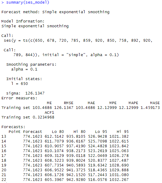
summary(ses_model)Result:
Holt’s Method (Double Exponential Smoothing)
Determine Holts method (double exponential smoothing) forecasts for periods 2-10 using a =0.6 and β =0.3, assuming L1 = D1 and T1 = D2 – D1
Excel
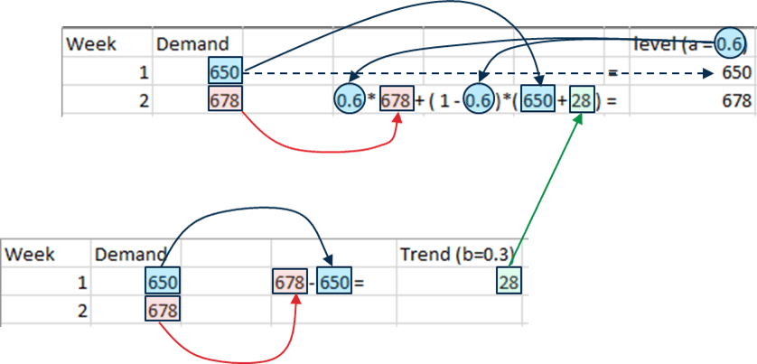


ps. Alpha value determine position value change and beta value determine slope change from one particular period to the next.
R
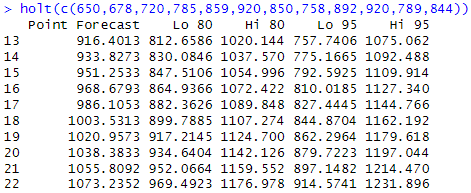
holt(data) → create Holt model
holt(c(650,678,720,785,859,920,850,758,892,920,789,844))Result:
plot(ts(c(650,678,720,785,859,920,850,758,892,920,789,844)),
     ylim=c(600,950))
lines(holt(c(650,678,720,785,859,920,850,758,892,920,789,844),
           initial="simple",
           alpha=0.6,
           beta=0.3)$fitted,
      col=2,
      lwd=2)
Result:

ps. somehow unable to achieve Excel result; no clear explanation how to use the function in R.
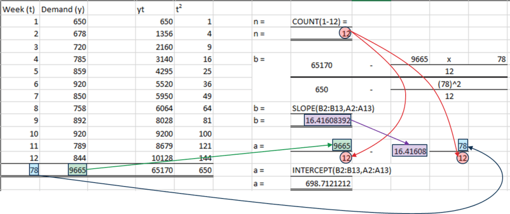
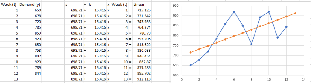
Linear / Quadratic / Exponential Trend
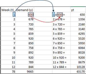
Step 1. Calculate multiplication, y x t
Step 2. Calculate t power 2


Step 3. Sum for all 4 column

R
tslm(data) → create linear regression time series forecast model
demand = ts(c(650,678,720,785,859,920,850,758,892,920,789,844))
time = 1:12
linear_model = tslm(demand~time)
Result:

plot(demand)
lines(linear_model$fitted.values,
      col=2,
      lwd=2)
Result:

Decomposition Model
Similar to merging 2 mathematical operation, but decomposition; separate seasonal variation and trend variation.
However, decompose require us with pre-requisite knowledge of choosing additive or multiplicative
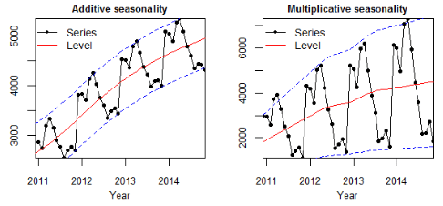
| a time series with constant variability | a time series with variability increasing with trend |
| deviation from the trend is fairly stable |
Excel (Additive)
Step 1. Calculate 4-MA
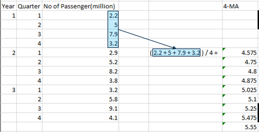

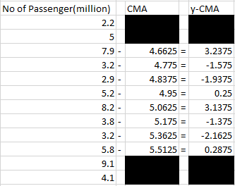
Step 2. Calculate CMA (center moving average) from 4-MA. Note that this is actually forming the “Trend Component”.
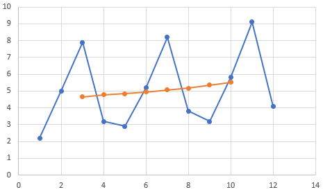
As the dataset was even number, CMA was performed for getting the center.
Step 3. Calculate y-CMA. Note. this part means that seasonal component are independent from each other, vary around 0 (i.e: trend-cycle will not cause an increase in the magnitude of seasonality).

Step 4. Fill up Seasonal table. In this scenario, 4 column represent 4 quarter, it could be 12 column for month.
Step 5. Perform total and using it to formulate average. Note that average in this scenario was divided by 2 as each column only has 2 value. DO NOTE put zero in Y1Q1, Y1Q2, Y3Q3, Y3Q4.
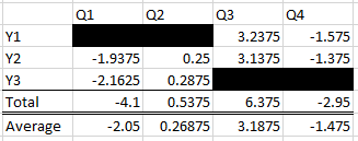

Adjusted

Step 6. Check if total of average are equal to zero, compensate if not. Note that this is actually forming the “Seasonal Component”.
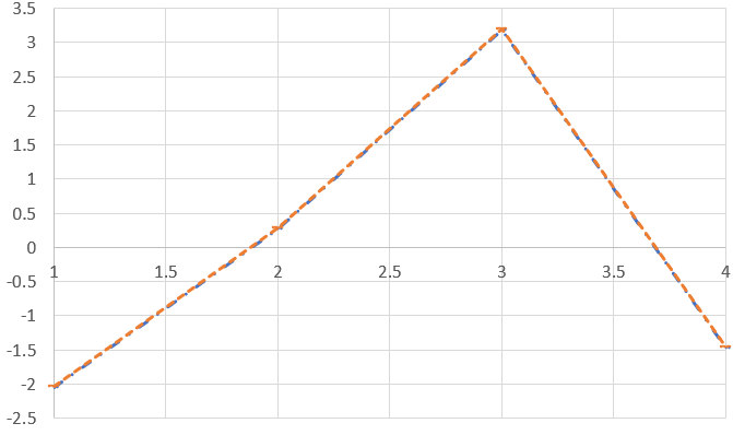
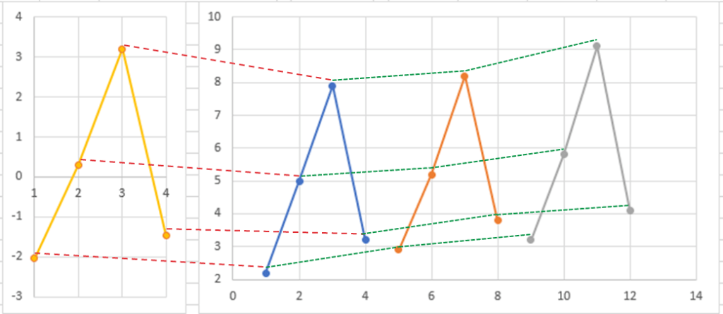
Step 7. Calculate subsequence value of CMA using slope and indexes. Add it with seasonal table data.
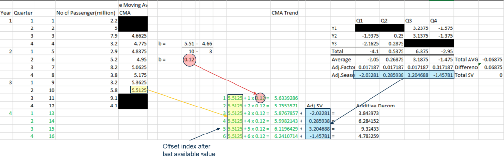
Step 7 (1). Linear Regression can be use as Trend component if needed.
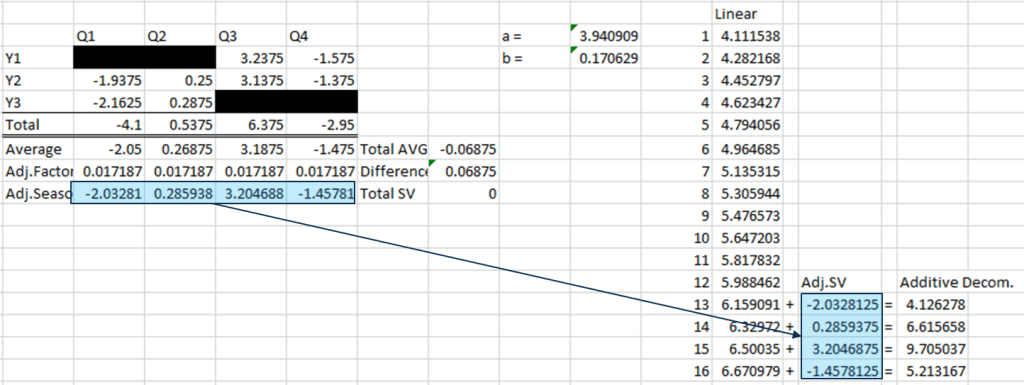
Result:

Excel (Multiplicative)
Continue from step 3 from Additive Decomposition Model.
Step 3. Calculate y-CMA
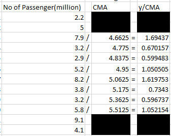

Proceed with Additive Decomposition Model Step 4, 5, 6. Take note that instead of compensate to reach zero, Multiplicative require four (each season contribute one).
Step 7. Instead like Additive Decomposition Model, multiply Trend with Seasonal.

Result:
R
decompose(data) → breakdown time series into trend, seasonality and random
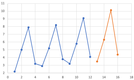
passanger = ts(c(2.2,5,7.9,3.2,2.9,5.2,8.2,3.8,3.2,5.8,9.1,4.1),
               frequency=4)
plot(decompose(passanger))
Result:

plot(passanger)
lines(stlm(passanger)$fitted,
      col=2,
      lwd=2)
Result:


Leave a comment